
Polar Equations
by
Susan Sexton
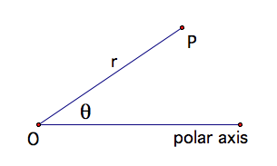
The polar coordinate system
uses distances and directions to specify the locations of points in the
plane. If P is any point in the plane then its location in the
plane is its distance from a fixed point called O (the origin) or the pole and its angle measurement from a horizontal axis
called the polar axis. The distance from O is denoted as r and the angle measurement from the polar axis is ![]() . Therefore the
location of P is represented by (r,
. Therefore the
location of P is represented by (r, ![]() ) as illustrated in the figure below.
) as illustrated in the figure below.
What would the graph of a
polar equation look like? It would
consist of all the points, P, that
satisfy the equation ![]() .
.
How can we compare this to
our usual rectangular form? If P is a point in the Cartesian plane then its
coordinates are (x, y). To plot P in the polar plane then ![]() and
and ![]() as illustrated
in the figure below.
as illustrated
in the figure below.
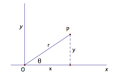
Notice that we have a right
triangle so we can use the Pythagorean Theorem to find r, x or y in the
equation: ![]() .
.
Let’s explore some graphs of
polar equations.
Consider the polar equation:
![]()
What happens when k is varied and a and b are fixed? For the
exploration I will let a and b be 1.
![]()
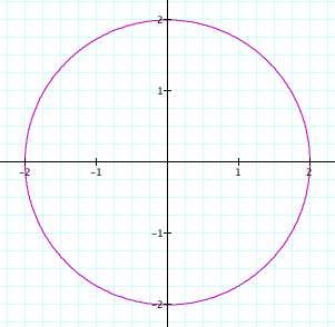
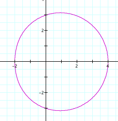
Why would this be a circle? Since cos 0 = 1 then we have ![]() so
so ![]() . So no matter
what
. So no matter
what ![]() is the graph
will be the set of points 2 units away from the origin.
is the graph
will be the set of points 2 units away from the origin.
![]()

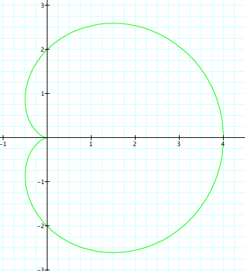
The graph is a special type of limacon, a
cardioid.
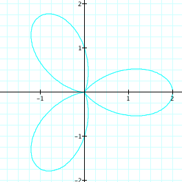
![]()
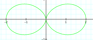
The graph is a 2 pedal rose.
![]()
The graph is a 3 pedal rose.
What do you think the graph will look like when k = 4 or k
= 5?
![]()
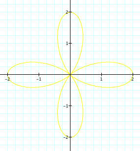
![]()
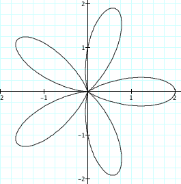
The graphs are 4 pedal and 5 pedal roses
respectfully!
What can we say about the effect of k on the graph?
It determines the number of pedals.
Looking at the graphs explored above, it appears that
their domains and ranges were both between -2 and 2. Lets see them all on the same graph.
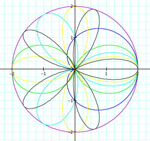
So the circle with r = 2 is the boundary
for any of the graphs of
![]() .
.
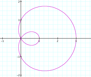
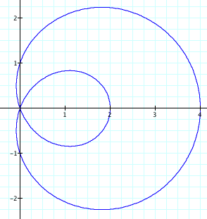
Let us now move on to varying a and b
and leaving k fixed.
![]()
![]()
![]()
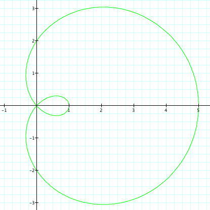
In each of three previous graphs we had a < b
and all resulted in a special type of limacon,
one with an inner loop.
What would happen if a = b?
(We’ve already seen one example!)
![]()
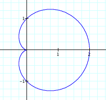
![]()
Same type of graph, lets see what happens when a > b.
![]()
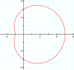
This graph is again a special type of limacon, a
“dimpled” one.
![]()
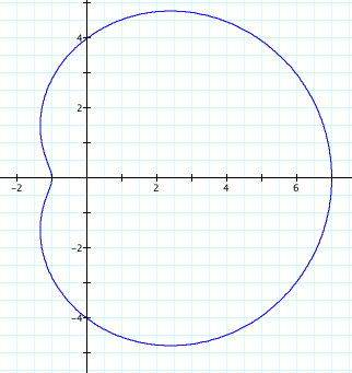
Still gives us a dimpled limacon.
![]()
Wait!
What happened to the dimple?
This graph is a result of a > 2b
and it is called a convex limacon.
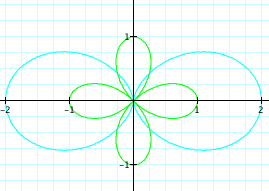
Let’s now compare
![]()
to
![]() .
.
We can use the
equations of the graphs explored earlier.
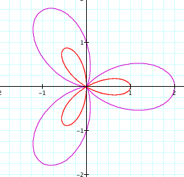
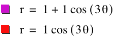
Interesting, when k is odd, the graph yielded the
same number of leaves.
When k is even the new graph had double
the number of leaves.
Lets explore a couple more
to see if this holds.
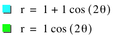
So it holds!
What happens when cosine is replaced by sine?
Lets look at the initial graphs
explored all at once.
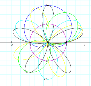
The graphs' orientation is certainly different!
Also when k = 0 the graph of the circle is a unit circle!
It is no longer the boundary of the
other graphs.
Discussion:
There are some interesting things running through this exploration.
Some ideas to consider for further exploration might be:
Why does sine affect the
graphs?
Why does k affect the graphs?
Are there other type of
polar curves that exist but not yet seen due to the type of equations we have
explored thus far?
What happens when a, b,
and k become negative integers?